Artificial Inteligence

Author

Affiliations

Md Rasheduzzaman

FLI Insel Riems

& Freelancer

Last updated

September 26, 2025

Content summary

Tensor, etc.

Tensor and PyTorch

Let’s load pytorch library and see the version of it.

import torch
print(torch.__version__)

2.7.0

Use CPU if GPU (CUDA) is not available.

if torch.cuda.is_available():
    print("GPU is available!")
    print(f"Using GPU: {torch.cuda.get_device_name(0)}")
else:
    print("GPU not available. Using CPU.")

GPU not available. Using CPU.

So, I am using CPU. Let’s start making tensors and build from very basics.

Tensor Creation

# using empty
a = torch.empty(2,3)
a

tensor([[0., 0., 0.],
        [0., 0., 0.]])

Let’s check type of pur tensor.

# check type
type(a)

torch.Tensor

# using ones
torch.ones(3,3)

tensor([[1., 1., 1.],
        [1., 1., 1.],
        [1., 1., 1.]])

# using zeros
torch.zeros(3,3)

tensor([[0., 0., 0.],
        [0., 0., 0.],
        [0., 0., 0.]])

# using rand
torch.manual_seed(40)
torch.rand(2,3)

tensor([[0.3679, 0.8661, 0.1737],
        [0.7157, 0.8649, 0.4878]])

torch.manual_seed(40)
torch.rand(2,3)

tensor([[0.3679, 0.8661, 0.1737],
        [0.7157, 0.8649, 0.4878]])

torch.randint(size=(2,3), low=0, high=10, dtype=torch.float32)

tensor([[6., 3., 6.],
        [7., 6., 5.]])

# using tensor
torch.tensor([[3,2,1],[4,5,6]])

tensor([[3, 2, 1],
        [4, 5, 6]])

# other ways

# arange
a = torch.arange(0,15,3)
print("using arange ->", a)

# using linspace
b = torch.linspace(0,15,10)
print("using linspace ->", b)

# using eye
c = torch.eye(4)
print("using eye ->", c)

# using full
d = torch.full((3, 3), 5)
print("using full ->", d)

using arange -> tensor([ 0,  3,  6,  9, 12])
using linspace -> tensor([ 0.0000,  1.6667,  3.3333,  5.0000,  6.6667,  8.3333, 10.0000, 11.6667,
        13.3333, 15.0000])
using eye -> tensor([[1., 0., 0., 0.],
        [0., 1., 0., 0.],
        [0., 0., 1., 0.],
        [0., 0., 0., 1.]])
using full -> tensor([[5, 5, 5],
        [5, 5, 5],
        [5, 5, 5]])

Tensor shape

We are making a new tensor (x) and checking shape of it. We can use the shape of x or any other already created tensor to make new tensors of that shape.

x = torch.tensor([[1,2,3],[5,6,7]])
x

tensor([[1, 2, 3],
        [5, 6, 7]])

x.shape

torch.Size([2, 3])

torch.empty_like(x)

tensor([[0, 0, 0],
        [0, 0, 0]])

torch.zeros_like(x)

tensor([[0, 0, 0],
        [0, 0, 0]])

torch.rand_like(x)

RuntimeError: "check_uniform_bounds" not implemented for 'Long'

It’s not working, since rand makes float values in the tensor. So, we need to specify data type as float.

torch.rand_like(x, dtype=torch.float32)

tensor([[0.7583, 0.8896, 0.6959],
        [0.4810, 0.8545, 0.1130]])

Tensor Data Types

# find data type
x.dtype

torch.int64

We are changing data type from float to int using dtype here.

# assign data type
torch.tensor([1.0,2.0,3.0], dtype=torch.int32)

tensor([1, 2, 3], dtype=torch.int32)

Similarly, from int to float using dtype here.

torch.tensor([1,2,3], dtype=torch.float64)

tensor([1., 2., 3.], dtype=torch.float64)

#using to()
x.to(torch.float32)

tensor([[1., 2., 3.],
        [5., 6., 7.]])

Some common data types in torch:

Data Type	Dtype	Description
32-bit Floating Point	`torch.float32`	Standard floating-point type used for most deep learning tasks. Provides a balance between precision and memory usage.
64-bit Floating Point	`torch.float64`	Double-precision floating point. Useful for high-precision numerical tasks but uses more memory.
16-bit Floating Point	`torch.float16`	Half-precision floating point. Commonly used in mixed-precision training to reduce memory and computational overhead on modern GPUs.
BFloat16	`torch.bfloat16`	Brain floating-point format with reduced precision compared to `float16`. Used in mixed-precision training, especially on TPUs.
8-bit Floating Point	`torch.float8`	Ultra-low-precision floating point. Used for experimental applications and extreme memory-constrained environments (less common).
8-bit Integer	`torch.int8`	8-bit signed integer. Used for quantized models to save memory and computation in inference.
16-bit Integer	`torch.int16`	16-bit signed integer. Useful for special numerical tasks requiring intermediate precision.
32-bit Integer	`torch.int32`	Standard signed integer type. Commonly used for indexing and general-purpose numerical tasks.
64-bit Integer	`torch.int64`	Long integer type. Often used for large indexing arrays or for tasks involving large numbers.
8-bit Unsigned Integer	`torch.uint8`	8-bit unsigned integer. Commonly used for image data (e.g., pixel values between 0 and 255).
Boolean	`torch.bool`	Boolean type, stores `True` or `False` values. Often used for masks in logical operations.
Complex 64	`torch.complex64`	Complex number type with 32-bit real and 32-bit imaginary parts. Used for scientific and signal processing tasks.
Complex 128	`torch.complex128`	Complex number type with 64-bit real and 64-bit imaginary parts. Offers higher precision but uses more memory.
Quantized Integer	`torch.qint8`	Quantized signed 8-bit integer. Used in quantized models for efficient inference.
Quantized Unsigned Integer	`torch.quint8`	Quantized unsigned 8-bit integer. Often used for quantized tensors in image-related tasks.

Mathematical Operations

Scalar operation

Let’s define a tensor x first.

x = torch.rand(2, 3)
x

tensor([[0.6779, 0.0173, 0.1203],
        [0.1363, 0.8089, 0.8229]])

Now, let’s see some scalar operation on this tensor.

#addition
x + 2
#subtraction
x - 3
#multiplication
x*4
#division
x/2
#integer division
(x*40)//3
#modulus division
((x*40)//3)%2
#power
x**2

tensor([[4.5950e-01, 2.9987e-04, 1.4484e-02],
        [1.8587e-02, 6.5435e-01, 6.7723e-01]])

Element-wise operation

Let’s make 2 new tensors first. To do anything element-wise, the shape of the tensors should be the same.

a = torch.rand(2, 3)
b = torch.rand(2, 3)
print(a)
print(b)

tensor([[0.3759, 0.0295, 0.4132],
        [0.0791, 0.0489, 0.9287]])
tensor([[0.4924, 0.8416, 0.1756],
        [0.5687, 0.4447, 0.0310]])

#add
a + b
#subtract
a - b
#multiply
a*b
#division
a/b
#power
a**b
#mod
a%b
#int division
a//b

tensor([[ 0.,  0.,  2.],
        [ 0.,  0., 29.]])

Let’s apply absolute function on a custom tensor.

#abs
c = torch.tensor([-1, 2, -3, 4, -5, -6, 7, -8])
torch.abs(c)

tensor([1, 2, 3, 4, 5, 6, 7, 8])

We only have positive values, right? As expected.

Let’s apply negative on the tensor.

torch.neg(c)

tensor([ 1, -2,  3, -4,  5,  6, -7,  8])

We have negative signs on the previously positives, and positive signs on the previously negatives, right?

#round
d = torch.tensor([1.4, 4.4, 3.6, 3.01, 4.55, 4.9])
torch.round(d)
# ceil
torch.ceil(d)
# floor
torch.floor(d)

tensor([1., 4., 3., 3., 4., 4.])

Do you see what round, ciel, floor are doing here? It is not that difficult, try to see.

Let’s do some clamping. So, if a value is smaller than the min value provided, that value will be equal to the min value and values bigger than the max value will be made equal to the max value. All other values in between the range will be kept as they are.

# clamp
d
torch.clamp(d, min=2, max=4)

tensor([2.0000, 4.0000, 3.6000, 3.0100, 4.0000, 4.0000])

Reduction operation

e = torch.randint(size=(2,3), low=0, high=10, dtype=torch.float32)
e

tensor([[5., 1., 7.],
        [7., 1., 5.]])

# sum
torch.sum(e)
# sum along columns
torch.sum(e, dim=0)
# sum along rows
torch.sum(e, dim=1)
# mean
torch.mean(e)
# mean along col
torch.mean(e, dim=0)
# mean along row
torch.mean(e, dim=1)
# median
torch.median(e)
torch.median(e, dim=0)
torch.median(e, dim=1)

torch.return_types.median(
values=tensor([5., 5.]),
indices=tensor([0, 2]))

# max and min
torch.max(e)
torch.max(e, dim=0)
torch.max(e, dim=1)

torch.min(e)
torch.min(e, dim=0)
torch.min(e, dim=1)

torch.return_types.min(
values=tensor([1., 1.]),
indices=tensor([1, 1]))

# product
torch.prod(e)
#do yourself dimension-wise

tensor(1225.)

# standard deviation
torch.std(e)
#do yourself dimension-wise

tensor(2.7325)

# variance
torch.var(e)
#do yourself dimension-wise

tensor(7.4667)

Which value is the biggest here? How to get its position/index? Use argmax.

# argmax
torch.argmax(e)

tensor(2)

Which value is the smallest here? How to get its position/index? Use argmin.

# argmin
torch.argmin(e)

tensor(1)

Matrix operations

m1 = torch.randint(size=(2,3), low=0, high=10)
m2 = torch.randint(size=(3,2), low=0, high=10)

print(m1)
print(m2)

tensor([[8, 9, 1],
        [2, 4, 5]])
tensor([[6, 5],
        [6, 2],
        [0, 6]])

# matrix multiplcation
torch.matmul(m1, m2)

tensor([[102,  64],
        [ 36,  48]])

Dot products:

vector1 = torch.tensor([1, 2])
vector2 = torch.tensor([3, 4])

# dot product
torch.dot(vector1, vector2)

tensor(11)

# transpose
torch.transpose(m2, 0, 1)

tensor([[6, 6, 0],
        [5, 2, 6]])

h = torch.randint(size=(3,3), low=0, high=8, dtype=torch.float32)
h

tensor([[7., 1., 3.],
        [3., 2., 2.],
        [7., 2., 4.]])

# determinant
torch.det(h)

tensor(6.0000)

# inverse
torch.inverse(h)

tensor([[ 0.6667,  0.3333, -0.6667],
        [ 0.3333,  1.1667, -0.8333],
        [-1.3333, -1.1667,  1.8333]])

Comparison operations

i = torch.randint(size=(2,3), low=0, high=10)
j = torch.randint(size=(2,3), low=0, high=10)

print(i)
print(j)

tensor([[1, 0, 1],
        [7, 8, 9]])
tensor([[1, 9, 7],
        [4, 5, 9]])

# greater than
i > j
# less than
i < j
# equal to
i == j
# not equal to
i != j
# greater than equal to

# less than equal to

tensor([[False,  True,  True],
        [ True,  True, False]])

Special functions

k = torch.randint(size=(2,3), low=0, high=10, dtype=torch.float32)
k

tensor([[5., 8., 1.],
        [3., 4., 4.]])

# log
torch.log(k)

tensor([[1.6094, 2.0794, 0.0000],
        [1.0986, 1.3863, 1.3863]])

# exp
torch.exp(k)

tensor([[1.4841e+02, 2.9810e+03, 2.7183e+00],
        [2.0086e+01, 5.4598e+01, 5.4598e+01]])

# sqrt
torch.sqrt(k)

tensor([[2.2361, 2.8284, 1.0000],
        [1.7321, 2.0000, 2.0000]])

k
# sigmoid
torch.sigmoid(k)

tensor([[0.9933, 0.9997, 0.7311],
        [0.9526, 0.9820, 0.9820]])

k
# softmax
torch.softmax(k, dim=0)

tensor([[0.8808, 0.9820, 0.0474],
        [0.1192, 0.0180, 0.9526]])

# relu
torch.relu(k)

tensor([[5., 8., 1.],
        [3., 4., 4.]])

Inplace Operations

m = torch.rand(2,3)
n = torch.rand(2,3)

print(m)
print(n)

tensor([[0.2179, 0.5475, 0.4801],
        [0.2278, 0.7175, 0.8381]])
tensor([[0.2569, 0.9879, 0.0779],
        [0.3233, 0.7714, 0.9524]])

m.add_(n)
m
n

tensor([[0.2569, 0.9879, 0.0779],
        [0.3233, 0.7714, 0.9524]])

torch.relu(m)

tensor([[0.4748, 1.5353, 0.5580],
        [0.5511, 1.4889, 1.7905]])

m.relu_()
m

tensor([[0.4748, 1.5353, 0.5580],
        [0.5511, 1.4889, 1.7905]])

Copying a Tensor

a = torch.rand(2,3)
a

tensor([[0.1013, 0.2033, 0.2292],
        [0.6055, 0.3249, 0.9225]])

b = a
a
b

tensor([[0.1013, 0.2033, 0.2292],
        [0.6055, 0.3249, 0.9225]])

a[0][0] = 0
a

tensor([[0.0000, 0.2033, 0.2292],
        [0.6055, 0.3249, 0.9225]])

tensor([[0.0000, 0.2033, 0.2292],
        [0.6055, 0.3249, 0.9225]])

id(a)

4624181456

id(b)

4624181456

Better way of making a copy

b = a.clone()
a
b

tensor([[0.0000, 0.2033, 0.2292],
        [0.6055, 0.3249, 0.9225]])

a[0][0] = 10
a

tensor([[10.0000,  0.2033,  0.2292],
        [ 0.6055,  0.3249,  0.9225]])

tensor([[0.0000, 0.2033, 0.2292],
        [0.6055, 0.3249, 0.9225]])

Now, let’s check their memory locations. They are at different locations.

id(a)
id(b)

4624182608

Autograd

Let’s go hard way. Let’s define our own differentiation formula. Our equation was \(y = x^2\). So, the derivative \(\frac{dy}{dx}\) will be \(2x\).

def dy_dx(x):
  return 2*x

Let’s check for \(x = 3\) now.

dy_dx(3)

But using PyTorch, it will be easy.

#import torch
x = torch.tensor(3.0, requires_grad=True) #gradient calculation requirement is set as True
y = x**2
x
y

tensor(9., grad_fn=<PowBackward0>)

We need to use backward on the last calculation (or variable) though, to calculate the gradient.

y.backward()
x.grad

tensor(6.)

Now, let’s make the situation a bit complex. Let’s say we have another equation \(z = sin(y)\). So, if we want to calculate \(\frac{dz}{dx}\), it requires a chain formula to calculate the derivative. And it will be: \[\frac{dz}{dx} = \frac{dz}{dy}*\frac{dy}{dx}\]. If we solve the formula, the derivative will be: \(2*x*cos(x^2)\). And yes, since we have a trigonometric formula, we need to load the math library.

import math

def dz_dx(x):
    return 2 * x * math.cos(x**2)

dz_dx(2) #you can decide the value of your x here

-2.6145744834544478

But let’s use our friend PyTorch to make our life easier.

x = torch.tensor(2.0, requires_grad=True) #you can decide the value of your x here

y = x**2

z = torch.sin(y)
x
y
z

tensor(-0.7568, grad_fn=<SinBackward0>)

So, let’s use backward on our z.

z.backward()

x.grad

tensor(-2.6146)

y.grad

y.grad is not possible, since it is an intermediate leaf.

Real-world example:

Let’s say a student got CGPA 3.10 and did not get a placement in an institute. So, we can try to make a prediction.

import torch

# Inputs
x = torch.tensor(6.70)  # Input feature
y = torch.tensor(0.0)  # True label (binary)

w = torch.tensor(1.0)  # Weight
b = torch.tensor(0.0)  # Bias

# Binary Cross-Entropy Loss for scalar
def binary_cross_entropy_loss(prediction, target):
    epsilon = 1e-8  # To prevent log(0)
    prediction = torch.clamp(prediction, epsilon, 1 - epsilon)
    return -(target * torch.log(prediction) + (1 - target) * torch.log(1 - prediction))

# Forward pass
z = w * x + b  # Weighted sum (linear part)
y_pred = torch.sigmoid(z)  # Predicted probability

# Compute binary cross-entropy loss
loss = binary_cross_entropy_loss(y_pred, y)

# Derivatives:
# 1. dL/d(y_pred): Loss with respect to the prediction (y_pred)
dloss_dy_pred = (y_pred - y)/(y_pred*(1-y_pred))

# 2. dy_pred/dz: Prediction (y_pred) with respect to z (sigmoid derivative)
dy_pred_dz = y_pred * (1 - y_pred)

# 3. dz/dw and dz/db: z with respect to w and b
dz_dw = x  # dz/dw = x
dz_db = 1  # dz/db = 1 (bias contributes directly to z)

dL_dw = dloss_dy_pred * dy_pred_dz * dz_dw
dL_db = dloss_dy_pred * dy_pred_dz * dz_db

print(f"Manual Gradient of loss w.r.t weight (dw): {dL_dw}")
print(f"Manual Gradient of loss w.r.t bias (db): {dL_db}")

Manual Gradient of loss w.r.t weight (dw): 6.691762447357178
Manual Gradient of loss w.r.t bias (db): 0.998770534992218

But let’s use our friend again.

x = torch.tensor(6.7)
y = torch.tensor(0.0)

w = torch.tensor(1.0, requires_grad=True)
b = torch.tensor(0.0, requires_grad=True)
w
b

tensor(0., requires_grad=True)

z = w*x + b
z
y_pred = torch.sigmoid(z)
y_pred
loss = binary_cross_entropy_loss(y_pred, y)
loss

tensor(6.7012, grad_fn=<NegBackward0>)

loss.backward()

print(w.grad)
print(b.grad)

tensor(6.6918)
tensor(0.9988)

Let’s insert multiple values (or a vector).

x = torch.tensor([1.0, 2.0, 3.0], requires_grad=True)
x

tensor([1., 2., 3.], requires_grad=True)

y = (x**2).mean()
y

tensor(4.6667, grad_fn=<MeanBackward0>)

y.backward()
x.grad

tensor([0.6667, 1.3333, 2.0000])

If we rerun all these things, the values get updtaed. So, we need to stop this behavior. How to do it?

# clearing grad
x = torch.tensor(2.0, requires_grad=True)
x

tensor(2., requires_grad=True)

y = x ** 2
y

tensor(4., grad_fn=<PowBackward0>)

y.backward()

x.grad

tensor(4.)

x.grad.zero_()

tensor(0.)

Now, we don’t see requires_grad=True part here. So, it is off. Another way:

# option 1 - requires_grad_(False)
# option 2 - detach()
# option 3 - torch.no_grad()

x = torch.tensor(2.0, requires_grad=True)
x
x.requires_grad_(False)

tensor(2.)

y = x ** 2
y

tensor(4.)

#not possible now
y.backward()

RuntimeError: element 0 of tensors does not require grad and does not have a grad_fn

x = torch.tensor(2.0, requires_grad=True)
x

tensor(2., requires_grad=True)

z = x.detach()
z

tensor(2.)

y = x ** 2
y

tensor(4., grad_fn=<PowBackward0>)

y1 = z ** 2
y1

tensor(4.)

y.backward() #possible

y1.backward() #not possible

RuntimeError: element 0 of tensors does not require grad and does not have a grad_fn

PyTorch Trining Pipeline

import numpy as np
import pandas as pd
import torch
from sklearn.model_selection import train_test_split
from sklearn.preprocessing import StandardScaler
from sklearn.preprocessing import LabelEncoder

Load an example dataset

df = pd.read_csv('https://raw.githubusercontent.com/gscdit/Breast-Cancer-Detection/refs/heads/master/data.csv')
df.head()

	id	diagnosis	radius_mean	texture_mean	perimeter_mean	area_mean	smoothness_mean	compactness_mean	concavity_mean	concave points_mean	...	texture_worst	perimeter_worst	area_worst	smoothness_worst	compactness_worst	concavity_worst	concave points_worst	symmetry_worst	fractal_dimension_worst	Unnamed: 32
0	842302	M	17.99	10.38	122.80	1001.0	0.11840	0.27760	0.3001	0.14710	...	17.33	184.60	2019.0	0.1622	0.6656	0.7119	0.2654	0.4601	0.11890	NaN
1	842517	M	20.57	17.77	132.90	1326.0	0.08474	0.07864	0.0869	0.07017	...	23.41	158.80	1956.0	0.1238	0.1866	0.2416	0.1860	0.2750	0.08902	NaN
2	84300903	M	19.69	21.25	130.00	1203.0	0.10960	0.15990	0.1974	0.12790	...	25.53	152.50	1709.0	0.1444	0.4245	0.4504	0.2430	0.3613	0.08758	NaN
3	84348301	M	11.42	20.38	77.58	386.1	0.14250	0.28390	0.2414	0.10520	...	26.50	98.87	567.7	0.2098	0.8663	0.6869	0.2575	0.6638	0.17300	NaN
4	84358402	M	20.29	14.34	135.10	1297.0	0.10030	0.13280	0.1980	0.10430	...	16.67	152.20	1575.0	0.1374	0.2050	0.4000	0.1625	0.2364	0.07678	NaN

5 rows × 33 columns

df.shape

(569, 33)

df.drop(columns=['id', 'Unnamed: 32'], inplace= True)
df.head()

	diagnosis	radius_mean	texture_mean	perimeter_mean	area_mean	smoothness_mean	compactness_mean	concavity_mean	concave points_mean	symmetry_mean	...	radius_worst	texture_worst	perimeter_worst	area_worst	smoothness_worst	compactness_worst	concavity_worst	concave points_worst	symmetry_worst	fractal_dimension_worst
0	M	17.99	10.38	122.80	1001.0	0.11840	0.27760	0.3001	0.14710	0.2419	...	25.38	17.33	184.60	2019.0	0.1622	0.6656	0.7119	0.2654	0.4601	0.11890
1	M	20.57	17.77	132.90	1326.0	0.08474	0.07864	0.0869	0.07017	0.1812	...	24.99	23.41	158.80	1956.0	0.1238	0.1866	0.2416	0.1860	0.2750	0.08902
2	M	19.69	21.25	130.00	1203.0	0.10960	0.15990	0.1974	0.12790	0.2069	...	23.57	25.53	152.50	1709.0	0.1444	0.4245	0.4504	0.2430	0.3613	0.08758
3	M	11.42	20.38	77.58	386.1	0.14250	0.28390	0.2414	0.10520	0.2597	...	14.91	26.50	98.87	567.7	0.2098	0.8663	0.6869	0.2575	0.6638	0.17300
4	M	20.29	14.34	135.10	1297.0	0.10030	0.13280	0.1980	0.10430	0.1809	...	22.54	16.67	152.20	1575.0	0.1374	0.2050	0.4000	0.1625	0.2364	0.07678

5 rows × 31 columns

Train test split

X_train, X_test, y_train, y_test = train_test_split(df.iloc[:, 1:], df.iloc[:, 0], test_size=0.2)

Scaling

scaler = StandardScaler()
X_train = scaler.fit_transform(X_train)
X_test = scaler.transform(X_test)

X_train

array([[ 1.77838216,  0.33663923,  1.74213583, ...,  0.74198987,
         0.54222412, -1.11360554],
       [ 1.61664581,  0.24142272,  1.57193275, ...,  0.74198987,
        -0.55309099,  0.40465846],
       [ 0.16380724,  0.21123212,  0.12277511, ...,  0.73584429,
         0.23044292, -0.10326986],
       ...,
       [-0.0118719 ,  1.84152454, -0.01338735, ..., -0.12607243,
        -1.04116733, -0.04529978],
       [-1.07152384, -0.70609766, -1.02082747, ..., -0.23915099,
        -0.45678162,  0.7171448 ],
       [ 1.77001649,  0.59442051,  1.70566374, ...,  0.97552167,
        -0.45514925, -0.92092404]], shape=(455, 30))

y_train

533    M
517    M
16     M
101    B
109    B
      ..
207    M
419    B
560    B
320    B
365    M
Name: diagnosis, Length: 455, dtype: object

Label Encoding

encoder = LabelEncoder()
y_train = encoder.fit_transform(y_train)
y_test = encoder.transform(y_test)

y_train

array([1, 1, 1, 0, 0, 1, 0, 1, 0, 1, 1, 0, 0, 1, 0, 1, 0, 1, 0, 0, 0, 0,
       0, 0, 0, 0, 0, 0, 1, 1, 0, 1, 0, 1, 1, 0, 1, 0, 1, 0, 0, 0, 1, 0,
       1, 1, 0, 0, 1, 1, 0, 0, 0, 1, 0, 0, 0, 1, 0, 0, 0, 0, 1, 1, 1, 1,
       1, 1, 1, 0, 1, 0, 1, 1, 0, 0, 1, 0, 1, 0, 0, 1, 0, 1, 0, 0, 0, 0,
       0, 0, 0, 0, 0, 0, 1, 1, 0, 0, 0, 1, 1, 0, 0, 0, 1, 1, 1, 0, 0, 0,
       0, 1, 0, 1, 0, 0, 0, 0, 0, 1, 0, 0, 0, 1, 0, 0, 1, 0, 0, 0, 0, 1,
       0, 0, 1, 1, 0, 0, 0, 1, 0, 0, 1, 0, 1, 1, 1, 1, 0, 0, 0, 0, 0, 1,
       0, 0, 0, 1, 0, 1, 0, 1, 0, 0, 0, 0, 1, 0, 0, 1, 1, 0, 1, 0, 0, 0,
       0, 0, 0, 1, 1, 1, 0, 0, 0, 0, 0, 0, 0, 0, 0, 0, 1, 0, 1, 1, 1, 0,
       0, 0, 0, 1, 0, 0, 1, 0, 0, 1, 0, 0, 0, 0, 0, 0, 0, 1, 0, 0, 0, 1,
       1, 0, 0, 0, 0, 0, 1, 1, 0, 0, 0, 0, 1, 0, 1, 0, 0, 0, 0, 1, 0, 0,
       0, 0, 1, 0, 1, 0, 1, 0, 0, 0, 0, 0, 0, 0, 0, 0, 0, 0, 1, 0, 0, 1,
       0, 0, 0, 1, 1, 0, 0, 1, 1, 0, 1, 0, 1, 0, 1, 1, 1, 0, 1, 1, 0, 0,
       0, 1, 0, 0, 0, 0, 0, 0, 0, 0, 1, 0, 1, 1, 0, 1, 0, 0, 0, 0, 0, 0,
       1, 1, 1, 0, 1, 0, 0, 1, 1, 0, 1, 0, 0, 0, 0, 1, 0, 1, 0, 0, 0, 0,
       0, 0, 1, 1, 0, 0, 0, 1, 1, 1, 0, 0, 0, 0, 1, 0, 0, 1, 1, 0, 1, 0,
       1, 0, 0, 0, 1, 0, 0, 0, 0, 0, 1, 0, 0, 1, 1, 0, 1, 0, 1, 0, 0, 1,
       0, 0, 0, 1, 1, 0, 0, 0, 1, 1, 0, 0, 0, 0, 0, 0, 0, 0, 1, 1, 0, 1,
       1, 1, 0, 1, 1, 1, 1, 1, 0, 0, 0, 0, 0, 0, 1, 1, 1, 0, 0, 0, 0, 0,
       0, 1, 0, 0, 1, 0, 0, 0, 0, 0, 1, 1, 0, 0, 1, 0, 1, 1, 1, 1, 1, 0,
       0, 0, 0, 1, 1, 1, 0, 0, 1, 1, 1, 0, 0, 0, 1])

Numpy arrays to PyTorch tensors

X_train_tensor = torch.from_numpy(X_train)
X_test_tensor = torch.from_numpy(X_test)
y_train_tensor = torch.from_numpy(y_train)
y_test_tensor = torch.from_numpy(y_test)

X_train_tensor.shape

torch.Size([455, 30])

y_train_tensor.shape

torch.Size([455])

Defining the model

class MySimpleNN():

  def __init__(self, X):

    self.weights = torch.rand(X.shape[1], 1, dtype=torch.float64, requires_grad=True)
    self.bias = torch.zeros(1, dtype=torch.float64, requires_grad=True)

  def forward(self, X):
    z = torch.matmul(X, self.weights) + self.bias
    y_pred = torch.sigmoid(z)
    return y_pred

  def loss_function(self, y_pred, y):
    # Clamp predictions to avoid log(0)
    epsilon = 1e-7
    y_pred = torch.clamp(y_pred, epsilon, 1 - epsilon)

    # Calculate loss
    loss = -(y_train_tensor * torch.log(y_pred) + (1 - y_train_tensor) * torch.log(1 - y_pred)).mean()
    return loss

Important Parameters

learning_rate = 0.1
epochs = 25

Training Pipeline

# create model
model = MySimpleNN(X_train_tensor)

# define loop
for epoch in range(epochs):

  # forward pass
  y_pred = model.forward(X_train_tensor)

  # loss calculate
  loss = model.loss_function(y_pred, y_train_tensor)

  # backward pass
  loss.backward()

  # parameters update
  with torch.no_grad():
    model.weights -= learning_rate * model.weights.grad
    model.bias -= learning_rate * model.bias.grad

  # zero gradients
  model.weights.grad.zero_()
  model.bias.grad.zero_()

  # print loss in each epoch
  print(f'Epoch: {epoch + 1}, Loss: {loss.item()}')

Epoch: 1, Loss: 3.968025963705283
Epoch: 2, Loss: 3.864118509120392
Epoch: 3, Loss: 3.7541330076509594
Epoch: 4, Loss: 3.638331163567124
Epoch: 5, Loss: 3.5174341902058233
Epoch: 6, Loss: 3.3933643569290846
Epoch: 7, Loss: 3.2621320961969693
Epoch: 8, Loss: 3.1262147737756134
Epoch: 9, Loss: 2.988698930957073
Epoch: 10, Loss: 2.846942763920921
Epoch: 11, Loss: 2.6958299495752183
Epoch: 12, Loss: 2.5419935910597404
Epoch: 13, Loss: 2.3831413982619805
Epoch: 14, Loss: 2.2235735410390314
Epoch: 15, Loss: 2.066447122377066
Epoch: 16, Loss: 1.910431766057619
Epoch: 17, Loss: 1.7594278162011676
Epoch: 18, Loss: 1.6166291902936634
Epoch: 19, Loss: 1.4746437685958356
Epoch: 20, Loss: 1.3437662136173296
Epoch: 21, Loss: 1.2277088323530687
Epoch: 22, Loss: 1.1276737971797886
Epoch: 23, Loss: 1.0442162895988343
Epoch: 24, Loss: 0.9769917653527498
Epoch: 25, Loss: 0.9246446252633511

model.bias

tensor([-0.1058], dtype=torch.float64, requires_grad=True)

model.weights

tensor([[ 0.2628],
        [ 0.0059],
        [ 0.4382],
        [ 0.2972],
        [ 0.0064],
        [-0.6488],
        [-0.3415],
        [ 0.0583],
        [ 0.0673],
        [ 0.6336],
        [-0.0643],
        [ 0.4676],
        [ 0.1455],
        [ 0.3115],
        [ 0.1001],
        [-0.0605],
        [-0.2559],
        [ 0.3491],
        [ 0.6941],
        [-0.0211],
        [ 0.3778],
        [ 0.2139],
        [-0.5063],
        [ 0.0311],
        [ 0.3313],
        [-0.4985],
        [ 0.2924],
        [-0.0689],
        [ 0.0554],
        [ 0.3736]], dtype=torch.float64, requires_grad=True)

Evaluation

# model evaluation
with torch.no_grad():
  y_pred = model.forward(X_test_tensor)
  y_pred = (y_pred > 0.9).float()
  accuracy = (y_pred == y_test_tensor).float().mean()
  print(f'Accuracy: {accuracy.item()}')

Accuracy: 0.586334228515625

NN module

Dataset and DataLoader

ANN/MLP in PyTorch

We will use Fashion MNIST dataset for this purpose. We can find this dataset in Kaggle. It has 70,000 (28*28) fashion images. We will try to classify them using our ANN and improve our model. But we will use less images since we are using less local resource (CPU, not GPU).

Our ANN structure: 1 input layer with 28*28 = 784 nodes. Then we will have 2 hidden layers. The first one will have 128 neurons and the second one will have 64 neurons. Then we will have 1 output layer having 10 neurons. The hidden layers will use ReLU and the last output layer will use softmax since it is a multi-class classification problems. Workflow: - DataLoader object - Training loop - Evaluation

import pandas as pd
from sklearn.model_selection import train_test_split
import torch
from torch.utils.data import Dataset, DataLoader
import torch.nn as nn
import torch.optim as optim
import matplotlib.pyplot as plt

Now, after loading the packages, we can use them. Let’s make it reproducible using a seed.

torch.manual_seed(30)

<torch._C.Generator at 0x10f9c48f0>

# Use Fashion-MNIST from torchvision and create a small CSV
import torchvision
import torchvision.transforms as transforms
import numpy as np

# Download Fashion-MNIST
transform = transforms.Compose([transforms.ToTensor()])
fmnist = torchvision.datasets.FashionMNIST(root='./data', train=True, download=True, transform=transform)

# Create a small subset (first 1000 samples)
n_samples = 1000
images_list = []
labels_list = []

for i in range(min(n_samples, len(fmnist))):
    image, label = fmnist[i]
    # Convert tensor to numpy and flatten
    image_flat = image.numpy().flatten()
    images_list.append(image_flat)
    labels_list.append(label)

# Create DataFrame
images_array = np.array(images_list)
labels_array = np.array(labels_list)

# Combine labels and images
data = np.column_stack([labels_array, images_array])
columns = ['label'] + [f'pixel{i}' for i in range(784)]
df = pd.DataFrame(data, columns=columns)

# Save to CSV for future use
df.to_csv('fmnist_small.csv', index=False)
print(f"Created fmnist_small.csv with {len(df)} samples")

df.head()

Created fmnist_small.csv with 1000 samples

	label	pixel5	pixel8	...	pixel774	pixel775	pixel776	pixel777
0	9.0	0.000000	0.000000	...	0.000000	0.000000	0.000000	0.000000
1	0.0	0.003922	0.000000	...	0.466667	0.447059	0.509804	0.298039
2	0.0	0.000000	0.000000	...	0.000000	0.000000	0.003922	0.000000
3	3.0	0.000000	0.129412	...	0.000000	0.000000	0.000000	0.000000
4	0.0	0.000000	0.000000	...	0.000000	0.000000	0.000000	0.000000

5 rows × 785 columns

Let’s check some images.

# Create a 4x4 grid of images
fig, axes = plt.subplots(4, 4, figsize=(10, 10))
fig.suptitle("First 16 Images", fontsize=16)

# Plot the first 16 images from the dataset
for i, ax in enumerate(axes.flat):
    img = df.iloc[i, 1:].values.reshape(28, 28)  # Reshape to 28x28
    ax.imshow(img)  # Display in grayscale
    ax.axis('off')  # Remove axis for a cleaner look
    ax.set_title(f"Label: {df.iloc[i, 0]}")  # Show the label

plt.tight_layout(rect=[0, 0, 1, 0.96])  # Adjust layout to fit the title
plt.show()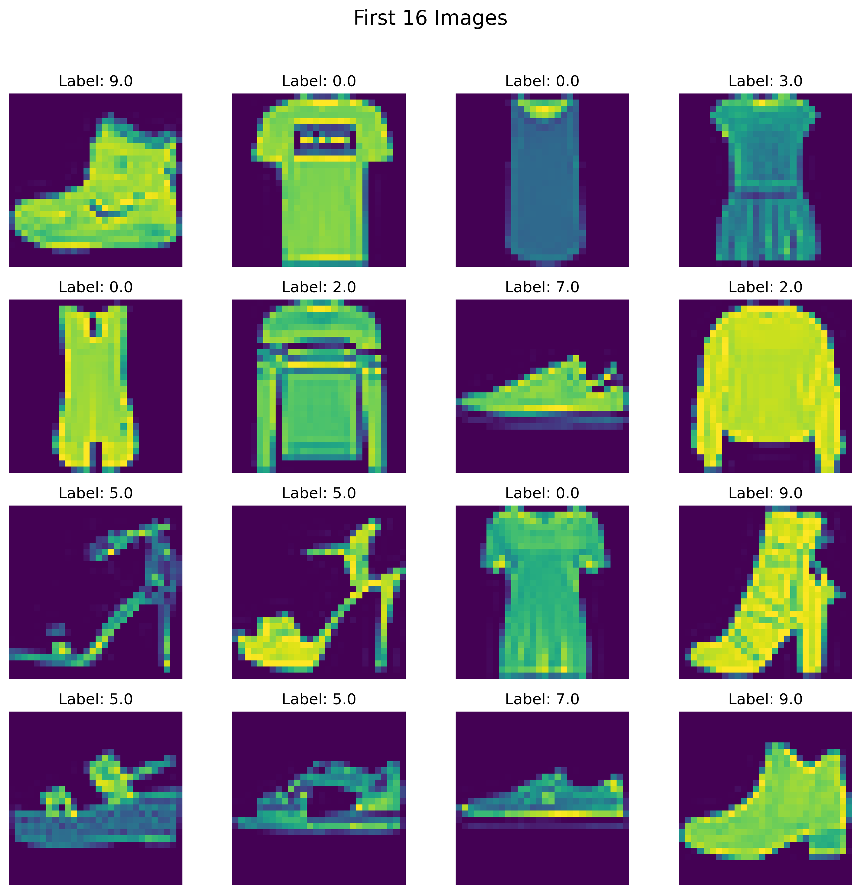

Citation

BibTeX citation:

@online{rasheduzzaman2025,
  author = {Md Rasheduzzaman},
  title = {Artificial {Inteligence}},
  date = {2025-09-26},
  langid = {en},
  abstract = {Tensor, etc.}
}

For attribution, please cite this work as:

Md Rasheduzzaman. 2025. “Artificial Inteligence.” September 26, 2025.