Statistics Basics

Author

Affiliations

Md Rasheduzzaman

FLI Insel Riems

& Freelancer

Content summary

Statistical tests, Statistics, Statistic, CLT, etc.

knitr::opts_chunk$set(echo = TRUE, warning = FALSE, message = FALSE, fig.width = 10, fig.height = 6)
library(tidyverse)
library(car)
library(emmeans)
library(knitr)
library(kableExtra)
library(patchwork)
library(corrplot)

# Helper function for separators
sep_line <- function(char = "=", n = 50) {
  cat(paste(rep(char, n), collapse = ""), "\n")
}

Part 1: The Coffee Shop Example - Why ANOVA Types Matter

Setting the Stage with a Simple Story

Imagine you own a coffee shop and want to understand what affects customer satisfaction scores (1-10 scale). You consider two factors:

1. Coffee Type: Regular vs Decaf
2. Time of Day: Morning vs Afternoon

Let’s create this scenario with data:

set.seed(42)

# Create a BALANCED design first (equal sample sizes)
n_per_cell <- 20  # 20 customers in each combination

balanced_coffee <- expand.grid(
  coffee_type = c("Regular", "Decaf"),
  time_of_day = c("Morning", "Afternoon"),
  replicate = 1:n_per_cell
) %>%
  mutate(
    # Create satisfaction scores with main effects and interaction
    satisfaction = case_when(
      coffee_type == "Regular" & time_of_day == "Morning" ~ rnorm(n(), 8, 1),    # High satisfaction
      coffee_type == "Regular" & time_of_day == "Afternoon" ~ rnorm(n(), 6, 1),  # Medium
      coffee_type == "Decaf" & time_of_day == "Morning" ~ rnorm(n(), 5, 1),      # Low-medium
      coffee_type == "Decaf" & time_of_day == "Afternoon" ~ rnorm(n(), 7, 1)     # Medium-high
    ),
    coffee_type = factor(coffee_type),
    time_of_day = factor(time_of_day)
  ) %>%
  select(-replicate)

# Show the structure
print("Balanced Design - Sample Sizes:")

[1] "Balanced Design - Sample Sizes:"

table(balanced_coffee$coffee_type, balanced_coffee$time_of_day)

         
          Morning Afternoon
  Regular      20        20
  Decaf        20        20

# Calculate means for each cell
cell_means_balanced <- balanced_coffee %>%
  group_by(coffee_type, time_of_day) %>%
  summarise(
    mean_satisfaction = mean(satisfaction),
    n = n(),
    .groups = 'drop'
  )

kable(cell_means_balanced, digits = 2, 
      caption = "Mean Satisfaction Scores - Balanced Design") %>%
  kable_styling(bootstrap_options = c("striped", "hover"))

Mean Satisfaction Scores - Balanced Design

coffee_type	time_of_day	mean_satisfaction	n
Regular	Morning	8.31	20
Regular	Afternoon	5.74	20
Decaf	Morning	5.00	20
Decaf	Afternoon	7.01	20

Now Let’s Create Reality: Unbalanced Data

In real life, you don’t get equal numbers of customers in each category. Maybe fewer people order decaf in the morning:

# Create UNBALANCED design (unequal sample sizes)
set.seed(42)

unbalanced_coffee <- bind_rows(
  # Regular + Morning: 30 customers (popular!)
  data.frame(
    coffee_type = "Regular",
    time_of_day = "Morning",
    satisfaction = rnorm(30, 8, 1)
  ),
  # Regular + Afternoon: 25 customers
  data.frame(
    coffee_type = "Regular",
    time_of_day = "Afternoon",
    satisfaction = rnorm(25, 6, 1)
  ),
  # Decaf + Morning: 10 customers (unpopular combination)
  data.frame(
    coffee_type = "Decaf",
    time_of_day = "Morning",
    satisfaction = rnorm(10, 5, 1)
  ),
  # Decaf + Afternoon: 20 customers
  data.frame(
    coffee_type = "Decaf",
    time_of_day = "Afternoon",
    satisfaction = rnorm(20, 7, 1)
  )
) %>%
  mutate(
    coffee_type = factor(coffee_type),
    time_of_day = factor(time_of_day)
  )

print("Unbalanced Design - Sample Sizes:")

[1] "Unbalanced Design - Sample Sizes:"

table(unbalanced_coffee$coffee_type, unbalanced_coffee$time_of_day)

         
          Afternoon Morning
  Decaf          20      10
  Regular        25      30

cell_means_unbalanced <- unbalanced_coffee %>%
  group_by(coffee_type, time_of_day) %>%
  summarise(
    mean_satisfaction = mean(satisfaction),
    n = n(),
    .groups = 'drop'
  )

kable(cell_means_unbalanced, digits = 2,
      caption = "Mean Satisfaction Scores - Unbalanced Design") %>%
  kable_styling(bootstrap_options = c("striped", "hover"))

Mean Satisfaction Scores - Unbalanced Design

coffee_type	time_of_day	mean_satisfaction	n
Decaf	Afternoon	7.13	20
Decaf	Morning	4.94	10
Regular	Afternoon	5.92	25
Regular	Morning	8.07	30

Part 2: The Mathematical Foundation of ANOVA

The General Linear Model

ANOVA is actually a special case of linear regression. Our two-way ANOVA model can be written as:

\[Y_{ijk} = \mu + \alpha_i + \beta_j + (\alpha\beta)_{ij} + \epsilon_{ijk}\]

Where:

• \(Y_{ijk}\) = satisfaction score for the \(k\)-th customer with coffee type \(i\) and time \(j\)
• \(\mu\) = grand mean (overall average satisfaction)
• \(\alpha_i\) = main effect of coffee type \(i\) (how much Regular or Decaf changes satisfaction)
• \(\beta_j\) = main effect of time of day \(j\) (how much Morning or Afternoon changes satisfaction)
• \((\alpha\beta)_{ij}\) = interaction effect (does the coffee type effect depend on time of day?)
• \(\epsilon_{ijk}\) = random error (individual differences)

Sum of Squares Decomposition

The total variation in our data can be decomposed:

\[SS_{Total} = SS_{CoffeeType} + SS_{Time} + SS_{Interaction} + SS_{Error}\]

In plain English: Total variation = Variation due to coffee type + Variation due to time + Variation due to their combination + Random variation

Part 3: Why Order Matters - A Visual Explanation

Understanding Sequential vs Simultaneous Testing

# Create a visual demonstration of why order matters
set.seed(123)

# Function to calculate partial correlations and visualize
demonstrate_order_effects <- function(data) {
  # Calculate total sum of squares
  grand_mean <- mean(data$satisfaction)
  ss_total <- sum((data$satisfaction - grand_mean)^2)
  
  # Calculate group means
  coffee_means <- tapply(data$satisfaction, data$coffee_type, mean)
  time_means <- tapply(data$satisfaction, data$time_of_day, mean)
  
  # Calculate marginal sums of squares (ignoring the other factor)
  ss_coffee_alone <- sum(table(data$coffee_type) * (coffee_means - grand_mean)^2)
  ss_time_alone <- sum(table(data$time_of_day) * (time_means - grand_mean)^2)
  
  # Create a data frame for visualization
  results <- data.frame(
    Approach = c("Coffee First", "Time First", "Coffee Alone", "Time Alone"),
    Coffee_SS = c(ss_coffee_alone, NA, ss_coffee_alone, NA),
    Time_SS = c(NA, ss_time_alone, NA, ss_time_alone),
    Order = c("1st", "1st", "Marginal", "Marginal")
  )
  
  return(list(
    ss_total = ss_total,
    ss_coffee_alone = ss_coffee_alone,
    ss_time_alone = ss_time_alone,
    coffee_means = coffee_means,
    time_means = time_means,
    grand_mean = grand_mean
  ))
}

# Apply to both datasets
balanced_results <- demonstrate_order_effects(balanced_coffee)
unbalanced_results <- demonstrate_order_effects(unbalanced_coffee)

# Create comparison table
comparison_df <- data.frame(
  Design = c("Balanced", "Balanced", "Unbalanced", "Unbalanced"),
  Factor = c("Coffee Type", "Time of Day", "Coffee Type", "Time of Day"),
  `SS When Tested First` = c(
    balanced_results$ss_coffee_alone,
    balanced_results$ss_time_alone,
    unbalanced_results$ss_coffee_alone,
    unbalanced_results$ss_time_alone
  ),
  check.names = FALSE
)

kable(comparison_df, digits = 2, 
      caption = "Sum of Squares When Each Factor is Tested First") %>%
  kable_styling(bootstrap_options = c("striped", "hover"))

Sum of Squares When Each Factor is Tested First

Design	Factor	SS When Tested First
Balanced	Coffee Type	21.03
Balanced	Time of Day	1.60
Unbalanced	Coffee Type	9.21
Unbalanced	Time of Day	14.48

Why Does Order Matter in Unbalanced Designs?

In unbalanced designs, the factors are correlated. When factors are correlated:

1. The effect of Coffee Type partially overlaps with the effect of Time
2. Testing Coffee first “claims” the overlapping variance
3. Testing Time first would claim that same overlapping variance differently
4. This is why Type I (sequential) ANOVA gives different results based on order

Part 4: The Controversy - Types I, II, and III Sum of Squares

Manual Calculation Tables for Understanding

Let’s manually calculate the different types of sum of squares to truly understand what’s happening:

# Function to manually calculate all types of SS
calculate_all_ss_types <- function(data, show_details = TRUE) {
  # Prepare data
  n <- nrow(data)
  grand_mean <- mean(data$satisfaction)
  
  # Get cell means and counts
  cell_summary <- data %>%
    group_by(coffee_type, time_of_day) %>%
    summarise(
      mean = mean(satisfaction),
      n = n(),
      sum = sum(satisfaction),
      .groups = 'drop'
    )
  
  # Marginal means
  coffee_marginal <- data %>%
    group_by(coffee_type) %>%
    summarise(
      mean = mean(satisfaction),
      n = n(),
      .groups = 'drop'
    )
  
  time_marginal <- data %>%
    group_by(time_of_day) %>%
    summarise(
      mean = mean(satisfaction),
      n = n(),
      .groups = 'drop'
    )
  
  if(show_details) {
    print("Cell Means and Sample Sizes:")
    print(cell_summary)
    print("")
    print("Marginal Means - Coffee Type:")
    print(coffee_marginal)
    print("")
    print("Marginal Means - Time of Day:")
    print(time_marginal)
    print("")
    print(paste("Grand Mean:", round(grand_mean, 3)))
    sep_line("-", 40)
  }
  
  # Calculate Type I SS (Sequential)
  # Order 1: Coffee -> Time -> Interaction
  
  # SS(Coffee | μ)
  ss_coffee_type1 <- sum(coffee_marginal$n * (coffee_marginal$mean - grand_mean)^2)
  
  # For SS(Time | μ, Coffee), we need residuals after fitting Coffee
  model_coffee_only <- lm(satisfaction ~ coffee_type, data = data)
  residuals_after_coffee <- residuals(model_coffee_only)
  
  # Create pseudo-data with residuals
  pseudo_data_time <- data.frame(
    residuals = residuals_after_coffee,
    time_of_day = data$time_of_day
  )
  
  model_time_on_residuals <- lm(residuals ~ time_of_day, data = pseudo_data_time)
  ss_time_type1 <- sum((fitted(model_time_on_residuals))^2)
  
  # Calculate Type II SS (Marginal, no interaction)
  model_both_main <- lm(satisfaction ~ coffee_type + time_of_day, data = data)
  model_coffee_only <- lm(satisfaction ~ coffee_type, data = data)
  model_time_only <- lm(satisfaction ~ time_of_day, data = data)
  
  ss_coffee_type2 <- sum((fitted(model_both_main) - fitted(model_time_only))^2)
  ss_time_type2 <- sum((fitted(model_both_main) - fitted(model_coffee_only))^2)
  
  # Calculate Type III SS (Marginal, with interaction)
  # This requires more complex calculations with contrast coding
  
  # Create results table
  results <- data.frame(
    `Type` = c("Type I", "Type II", "Type III*"),
    `SS_Coffee` = c(ss_coffee_type1, ss_coffee_type2, NA),
    `SS_Time` = c(ss_time_type1, ss_time_type2, NA),
    check.names = FALSE
  )
  
  return(results)
}

# Calculate for both designs
print("BALANCED DESIGN:")

[1] "BALANCED DESIGN:"

balanced_calc <- calculate_all_ss_types(balanced_coffee, show_details = TRUE)

[1] "Cell Means and Sample Sizes:"
# A tibble: 4 × 5
  coffee_type time_of_day  mean     n   sum
  <fct>       <fct>       <dbl> <int> <dbl>
1 Regular     Morning      8.31    20  166.
2 Regular     Afternoon    5.74    20  115.
3 Decaf       Morning      5.00    20  100.
4 Decaf       Afternoon    7.01    20  140.
[1] ""
[1] "Marginal Means - Coffee Type:"
# A tibble: 2 × 3
  coffee_type  mean     n
  <fct>       <dbl> <int>
1 Regular      7.03    40
2 Decaf        6.00    40
[1] ""
[1] "Marginal Means - Time of Day:"
# A tibble: 2 × 3
  time_of_day  mean     n
  <fct>       <dbl> <int>
1 Morning      6.66    40
2 Afternoon    6.37    40
[1] ""
[1] "Grand Mean: 6.516"
---------------------------------------- 

kable(balanced_calc, digits = 2, 
      caption = "Manual SS Calculations - Balanced Design") %>%
  kable_styling(bootstrap_options = c("striped", "hover"))

Manual SS Calculations - Balanced Design

Type	SS_Coffee	SS_Time
Type I	21.03	1.6
Type II	21.03	1.6
Type III*	NA	NA

print("")

[1] ""

print("UNBALANCED DESIGN:")

[1] "UNBALANCED DESIGN:"

unbalanced_calc <- calculate_all_ss_types(unbalanced_coffee, show_details = TRUE)

[1] "Cell Means and Sample Sizes:"
# A tibble: 4 × 5
  coffee_type time_of_day  mean     n   sum
  <fct>       <fct>       <dbl> <int> <dbl>
1 Decaf       Afternoon    7.13    20 143. 
2 Decaf       Morning      4.94    10  49.4
3 Regular     Afternoon    5.92    25 148. 
4 Regular     Morning      8.07    30 242. 
[1] ""
[1] "Marginal Means - Coffee Type:"
# A tibble: 2 × 3
  coffee_type  mean     n
  <fct>       <dbl> <int>
1 Decaf        6.40    30
2 Regular      7.09    55
[1] ""
[1] "Marginal Means - Time of Day:"
# A tibble: 2 × 3
  time_of_day  mean     n
  <fct>       <dbl> <int>
1 Afternoon    6.46    45
2 Morning      7.29    40
[1] ""
[1] "Grand Mean: 6.849"
---------------------------------------- 

kable(unbalanced_calc, digits = 2,
      caption = "Manual SS Calculations - Unbalanced Design") %>%
  kable_styling(bootstrap_options = c("striped", "hover"))

Manual SS Calculations - Unbalanced Design

Type	SS_Coffee	SS_Time
Type I	9.21	10.17
Type II	5.34	10.61
Type III*	NA	NA

Type I Sum of Squares (Sequential)

Mathematical Definition:

• \(SS(\alpha | \mu)\) = Sum of squares for A after fitting the mean
• \(SS(\beta | \mu, \alpha)\) = Sum of squares for B after fitting mean and A
• \(SS(\alpha\beta | \mu, \alpha, \beta)\) = Sum of squares for interaction after fitting everything else

Plain English: Type I asks “What does each factor explain that wasn’t already explained by factors entered before it?”

Example: When Type I Makes Sense

Scenario: Educational Achievement Study

Imagine studying factors affecting student test scores where we have a clear causal hierarchy:

1. Socioeconomic Status (SES) - This is a background variable that exists before schooling
2. School Quality - Students are assigned to schools based partly on where they live (related to SES)
3. Teaching Method - Applied within schools

Here, it makes sense to use Type I with SES entered first, then School Quality, then Teaching Method. We want to know:

• How much variance does SES explain?
• How much additional variance does School Quality explain after accounting for SES?
• How much additional variance does Teaching Method explain after accounting for both?

This sequential approach respects the causal/temporal ordering of these factors.

# Type I implementation with detailed output
print("TYPE I - Sequential Sum of Squares")

[1] "TYPE I - Sequential Sum of Squares"

sep_line("=", 50)

================================================== 

model_type1 <- lm(satisfaction ~ coffee_type + time_of_day + coffee_type:time_of_day, 
                  data = unbalanced_coffee)
anova_type1 <- anova(model_type1)
print(anova_type1)

Analysis of Variance Table

Response: satisfaction
                        Df Sum Sq Mean Sq F value    Pr(>F)    
coffee_type              1  9.214   9.214  7.9036  0.006186 ** 
time_of_day              1 10.607  10.607  9.0985  0.003417 ** 
coffee_type:time_of_day  1 84.400  84.400 72.3995 7.439e-13 ***
Residuals               81 94.426   1.166                      
---
Signif. codes:  0 '***' 0.001 '**' 0.01 '*' 0.05 '.' 0.1 ' ' 1

What Does Each Row Mean?

Click below to understand each row in the ANOVA table:

Click to see explanation

Row 1 - coffee_type: This shows the sum of squares for coffee type when it’s the FIRST factor considered (after the intercept). It answers: “How much variance in satisfaction is explained by coffee type alone?”

Row 2 - time_of_day: This shows the sum of squares for time of day AFTER removing the effect of coffee type. It answers: “How much additional variance is explained by time of day that wasn’t already explained by coffee type?”

Row 3 - coffee_type:time_of_day: This is the interaction term. It answers: “Is the effect of coffee type different at different times of day?” A significant interaction means the effect of one factor depends on the level of the other.

Row 4 - Residuals: This is the unexplained variance - the variation in satisfaction scores that can’t be explained by any of our factors. It represents individual differences and measurement error.

Columns Explained:

• Df (Degrees of Freedom): Number of independent pieces of information. For factors: (number of levels - 1)
• Sum Sq: Total squared deviations explained by that factor
• Mean Sq: Sum Sq divided by Df (average squared deviation)
• F value: Ratio of factor’s Mean Sq to Residual Mean Sq (signal-to-noise ratio)
• Pr(>F): p-value - probability of seeing this F-value or larger if null hypothesis is true

Type II Sum of Squares (Hierarchical)

Mathematical Definition:

• \(SS(\alpha | \mu, \beta)\) = Sum of squares for A after fitting mean and B
• \(SS(\beta | \mu, \alpha)\) = Sum of squares for B after fitting mean and A
• \(SS(\alpha\beta | \mu, \alpha, \beta)\) = Sum of squares for interaction after main effects

Plain English: Type II asks “What does each main effect explain that the other main effect doesn’t, ignoring interactions?”

When to use: When you want to test main effects assuming no interaction (most common in practice)

print("TYPE II - Hierarchical Sum of Squares")

[1] "TYPE II - Hierarchical Sum of Squares"

sep_line("=", 50)

================================================== 

Anova(model_type1, type = "II")

Anova Table (Type II tests)

Response: satisfaction
                        Sum Sq Df F value    Pr(>F)    
coffee_type              5.339  1  4.5802  0.035352 *  
time_of_day             10.607  1  9.0985  0.003417 ** 
coffee_type:time_of_day 84.400  1 72.3995 7.439e-13 ***
Residuals               94.426 81                      
---
Signif. codes:  0 '***' 0.001 '**' 0.01 '*' 0.05 '.' 0.1 ' ' 1

What Does Each Row Mean in Type II?

Click to see explanation

Key Differences from Type I:

Row 1 - coffee_type: Now shows SS for coffee type AFTER adjusting for time_of_day (but NOT interaction). It answers: “What unique variance does coffee type explain that time doesn’t?”

Row 2 - time_of_day: Shows SS for time AFTER adjusting for coffee_type (but NOT interaction). It answers: “What unique variance does time explain that coffee type doesn’t?”

Row 3 - coffee_type:time_of_day: Same as Type I - interaction is always tested last.

Why Type II is Often Preferred:

• Tests each main effect controlling for other main effects
• Order doesn’t matter (unlike Type I)
• Assumes no interaction when testing main effects
• More balanced approach for most research questions

Type III Sum of Squares (Marginal)

Mathematical Definition:

• \(SS(\alpha | \mu, \beta, \alpha\beta)\) = Sum of squares for A after fitting everything else
• \(SS(\beta | \mu, \alpha, \alpha\beta)\) = Sum of squares for B after fitting everything else
• \(SS(\alpha\beta | \mu, \alpha, \beta)\) = Sum of squares for interaction after main effects

Plain English: Type III asks “What does each effect explain that isn’t explained by any other effect, including interactions?”

# Type III implementation
# IMPORTANT: Must use sum-to-zero contrasts for Type III
contrasts(unbalanced_coffee$coffee_type) <- contr.sum(2)
contrasts(unbalanced_coffee$time_of_day) <- contr.sum(2)

model_type3 <- lm(satisfaction ~ coffee_type * time_of_day, data = unbalanced_coffee)

print("TYPE III - Marginal Sum of Squares")

[1] "TYPE III - Marginal Sum of Squares"

sep_line("=", 50)

================================================== 

Anova(model_type3, type = "III")

Anova Table (Type III tests)

Response: satisfaction
                         Sum Sq Df   F value    Pr(>F)    
(Intercept)             3041.77  1 2609.2756 < 2.2e-16 ***
coffee_type               16.40  1   14.0657 0.0003302 ***
time_of_day                0.01  1    0.0077 0.9302036    
coffee_type:time_of_day   84.40  1   72.3995 7.439e-13 ***
Residuals                 94.43 81                        
---
Signif. codes:  0 '***' 0.001 '**' 0.01 '*' 0.05 '.' 0.1 ' ' 1

What Does Each Row Mean in Type III?

Click to see explanation

Type III Special Characteristics:

Row 1 - (Intercept): Type III includes the intercept test, which tests if the grand mean equals zero (usually not interesting).

Row 2 - coffee_type: Tests coffee type AFTER adjusting for time AND interaction. Answers: “Is there a coffee type effect averaged across all times?”

Row 3 - time_of_day: Tests time AFTER adjusting for coffee type AND interaction. Answers: “Is there a time effect averaged across all coffee types?”

Row 4 - coffee_type:time_of_day: Same as other types - interaction effect.

When Type III is Useful:

• When interaction is significant
• When you want the most conservative test
• When following certain field conventions (e.g., some areas of psychology)
• Tests “average” effects across all levels of other factors

Part 5: Why All Three Types Give the Same Answer for Balanced Data

The Magic of Orthogonality

# Demonstrate orthogonality in balanced vs unbalanced designs

check_orthogonality <- function(data, title) {
  # Create design matrix
  X <- model.matrix(~ coffee_type * time_of_day, data = data)
  
  # Calculate correlation matrix (excluding intercept)
  cor_matrix <- cor(X[, -1])
  
  # Visualize
  par(mar = c(5, 4, 4, 2))
  corrplot(cor_matrix, 
           method = "color", 
           type = "upper",
           tl.cex = 0.8,
           tl.col = "black",
           title = title,
           mar = c(0, 0, 2, 0),
           addCoef.col = "black",
           number.cex = 0.8)
  
  return(cor_matrix)
}

# Check both designs
par(mfrow = c(1, 2))
balanced_cors <- check_orthogonality(balanced_coffee, 
                                     "Balanced Design\n(Orthogonal)")
unbalanced_cors <- check_orthogonality(unbalanced_coffee, 
                                       "Unbalanced Design\n(Non-orthogonal)")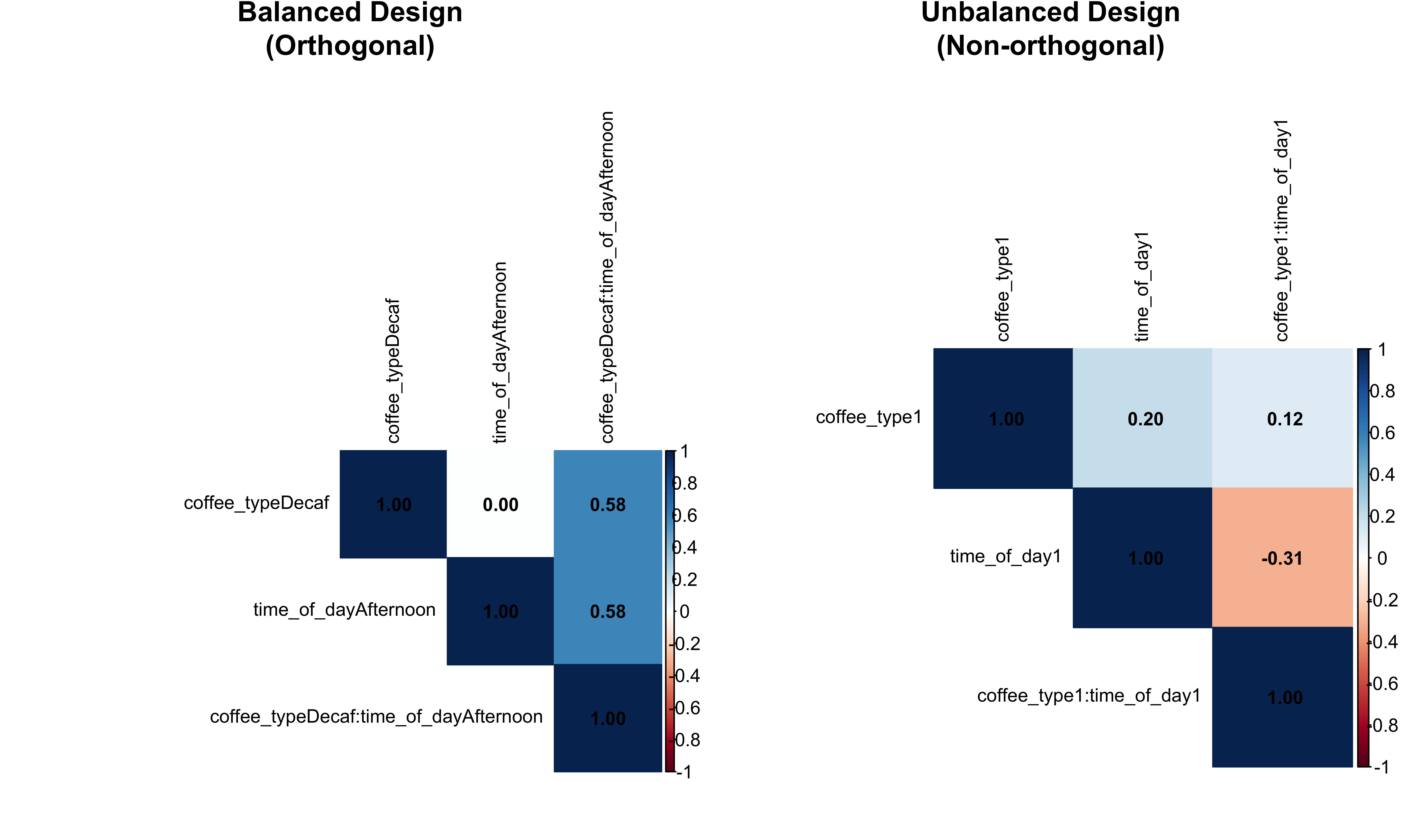

par(mfrow = c(1, 1))

Why Balanced Designs Make All Types Equal

In balanced designs, the design vectors are orthogonal (uncorrelated):

1. Zero Correlation: The correlation between coffee_type and time_of_day is 0
2. No Overlapping Variance: Each factor explains completely separate portions of variance
3. Order Doesn’t Matter: Since factors don’t overlap, the sequence of testing is irrelevant
4. Unique Contributions: Each factor’s contribution is unique and doesn’t depend on others

This is why balanced designs are so desirable in experimental research!

Detailed Comparison Table

# Create a comprehensive comparison
compare_ss_types <- function(data, design_name) {
  # Type I (two orders)
  model_i_order1 <- lm(satisfaction ~ coffee_type + time_of_day, data = data)
  model_i_order2 <- lm(satisfaction ~ time_of_day + coffee_type, data = data)
  
  type_i_order1 <- anova(model_i_order1)
  type_i_order2 <- anova(model_i_order2)
  
  # Type II
  type_ii <- Anova(model_i_order1, type = "II")
  
  # Type III (with proper contrasts)
  data_copy <- data
  contrasts(data_copy$coffee_type) <- contr.sum(2)
  contrasts(data_copy$time_of_day) <- contr.sum(2)
  model_iii <- lm(satisfaction ~ coffee_type + time_of_day, data = data_copy)
  type_iii <- Anova(model_iii, type = "III")
  
  # Create comparison table
  comparison <- data.frame(
    Design = design_name,
    Type = c("I (Coffee→Time)", "I (Time→Coffee)", "II", "III"),
    Coffee_SS = c(
      type_i_order1$`Sum Sq`[1],
      type_i_order2$`Sum Sq`[2],
      type_ii$`Sum Sq`[1],
      type_iii$`Sum Sq`[2]
    ),
    Time_SS = c(
      type_i_order1$`Sum Sq`[2],
      type_i_order2$`Sum Sq`[1],
      type_ii$`Sum Sq`[2],
      type_iii$`Sum Sq`[3]
    )
  )
  
  return(comparison)
}

# Compare both designs
balanced_comparison <- compare_ss_types(balanced_coffee, "Balanced")
unbalanced_comparison <- compare_ss_types(unbalanced_coffee, "Unbalanced")

full_comparison <- rbind(balanced_comparison, unbalanced_comparison)

kable(full_comparison, digits = 2,
      caption = "Sum of Squares Comparison: All Types, Both Designs") %>%
  kable_styling(bootstrap_options = c("striped", "hover")) %>%
  pack_rows("Balanced Design", 1, 4) %>%
  pack_rows("Unbalanced Design", 5, 8)

Sum of Squares Comparison: All Types, Both Designs

Design	Type	Coffee_SS	Time_SS
Balanced Design
Balanced	I (Coffee→Time)	21.03	1.60
Balanced	I (Time→Coffee)	21.03	1.60
Balanced	II	21.03	1.60
Balanced	III	21.03	1.60
Unbalanced Design
Unbalanced	I (Coffee→Time)	9.21	10.61
Unbalanced	I (Time→Coffee)	5.34	14.48
Unbalanced	II	5.34	10.61
Unbalanced	III	5.34	10.61

Part 6: Variance Heterogeneity (Unequal Variances)

Creating Data with Unequal Variances

set.seed(123)

# Create data with very different variances
hetero_data <- bind_rows(
  data.frame(
    group = "A",
    value = rnorm(30, mean = 50, sd = 2)  # Small variance
  ),
  data.frame(
    group = "B", 
    value = rnorm(30, mean = 52, sd = 8)  # Medium variance
  ),
  data.frame(
    group = "C",
    value = rnorm(30, mean = 54, sd = 15) # Large variance
  )
) %>%
  mutate(group = factor(group))

# Calculate actual variances
variance_summary <- hetero_data %>%
  group_by(group) %>%
  summarise(
    Mean = mean(value),
    Variance = var(value),
    SD = sd(value),
    n = n(),
    .groups = 'drop'
  )

kable(variance_summary, digits = 2,
      caption = "Group Statistics with Heterogeneous Variances") %>%
  kable_styling(bootstrap_options = c("striped", "hover"))

Group Statistics with Heterogeneous Variances

group	Mean	Variance	SD	n
A	49.91	3.85	1.96	30
B	53.43	44.64	6.68	30
C	54.37	170.22	13.05	30

# Visualize the different variances
p1 <- ggplot(hetero_data, aes(x = group, y = value, fill = group)) +
  geom_boxplot(alpha = 0.7) +
  geom_point(position = position_jitter(width = 0.1), alpha = 0.3) +
  labs(title = "Heterogeneous Variances",
       subtitle = "Notice the very different spreads") +
  theme_minimal()

p2 <- ggplot(hetero_data, aes(x = value, fill = group)) +
  geom_density(alpha = 0.5) +
  labs(title = "Density Plot", 
       subtitle = "Different widths = different variances") +
  theme_minimal()

p1 | p2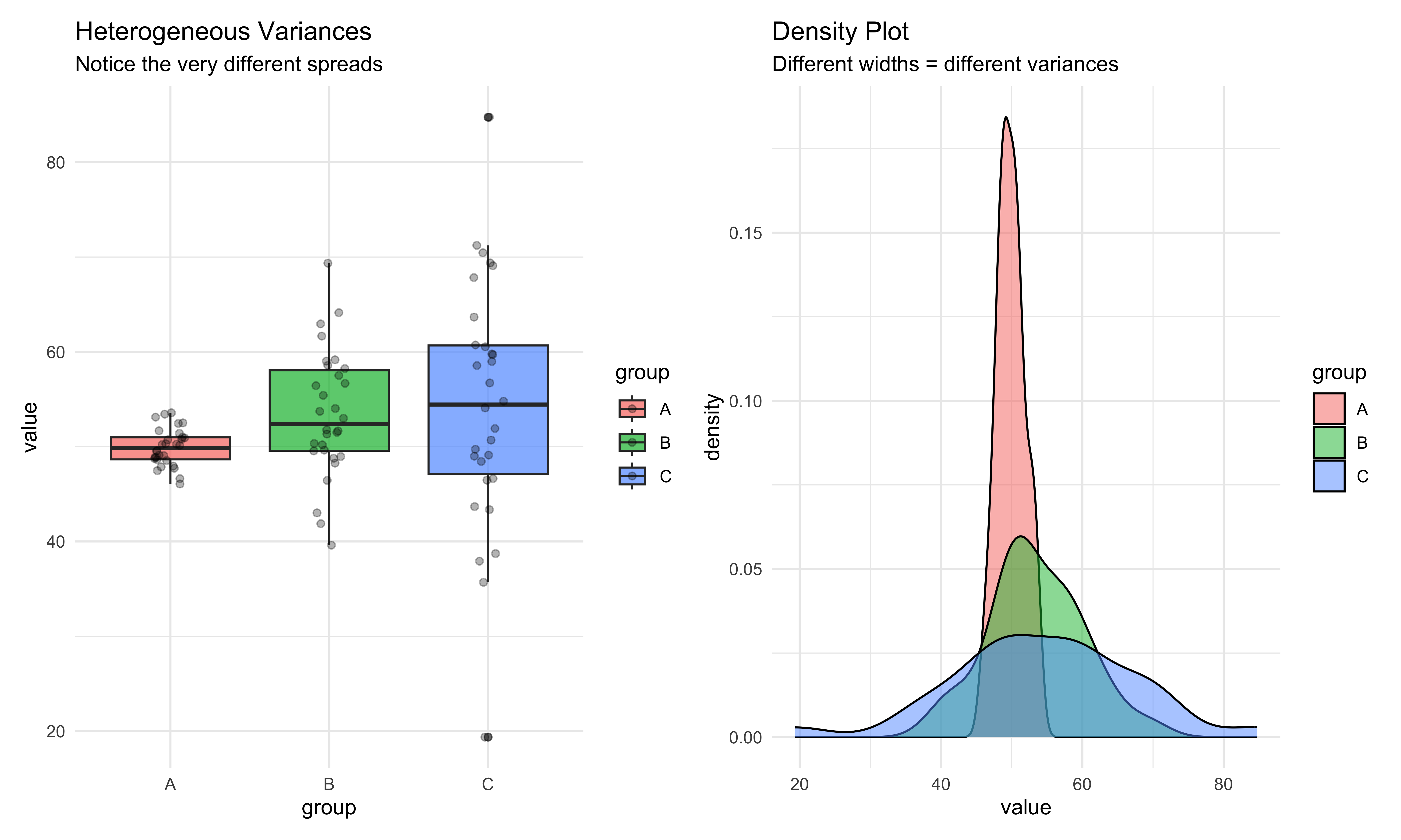

Testing for Homogeneity of Variance

print("Testing for Equal Variances:")

[1] "Testing for Equal Variances:"

sep_line("=", 50)

================================================== 

print("Levene's Test (robust to non-normality):")

[1] "Levene's Test (robust to non-normality):"

levene_test <- leveneTest(value ~ group, data = hetero_data)
print(levene_test)

Levene's Test for Homogeneity of Variance (center = median)
      Df F value  Pr(>F)    
group  2   19.13 1.3e-07 ***
      87                    
---
Signif. codes:  0 '***' 0.001 '**' 0.01 '*' 0.05 '.' 0.1 ' ' 1

print("")

[1] ""

print("Bartlett's Test (sensitive to non-normality):")

[1] "Bartlett's Test (sensitive to non-normality):"

bartlett_test <- bartlett.test(value ~ group, data = hetero_data)
print(bartlett_test)

    Bartlett test of homogeneity of variances

data:  value by group
Bartlett's K-squared = 73.797, df = 2, p-value < 2.2e-16

Interpreting Variance Tests

Levene’s Test: p < 0.05 indicates unequal variances (assumption violated)
Bartlett’s Test: More powerful but sensitive to non-normality

What to do with unequal variances:

1. Use Welch’s ANOVA instead of standard ANOVA
2. Use Games-Howell post-hoc test instead of Tukey
3. Consider transforming data (log, square root)
4. Use robust methods or non-parametric alternatives

Consequences of Ignoring Unequal Variances

# Standard ANOVA (assumes equal variances)
print("Standard ANOVA (assumes equal variances):")

[1] "Standard ANOVA (assumes equal variances):"

standard_anova <- aov(value ~ group, data = hetero_data)
summary(standard_anova)

            Df Sum Sq Mean Sq F value Pr(>F)
group        2    332   165.9   2.275  0.109
Residuals   87   6343    72.9               

print("")

[1] ""

print("Welch's ANOVA (robust to unequal variances):")

[1] "Welch's ANOVA (robust to unequal variances):"

welch_test <- oneway.test(value ~ group, data = hetero_data, var.equal = FALSE)
print(welch_test)

    One-way analysis of means (not assuming equal variances)

data:  value and group
F = 5.2616, num df = 2.000, denom df = 42.497, p-value = 0.009086

# Compare p-values
comparison_pvalues <- data.frame(
  Test = c("Standard ANOVA", "Welch's ANOVA"),
  `Assumes Equal Variances` = c("Yes", "No"),
  `p-value` = c(summary(standard_anova)[[1]]$`Pr(>F)`[1], welch_test$p.value),
  Decision = c(
    ifelse(summary(standard_anova)[[1]]$`Pr(>F)`[1] < 0.05, "Reject H0", "Fail to reject H0"),
    ifelse(welch_test$p.value < 0.05, "Reject H0", "Fail to reject H0")
  ),
  check.names = FALSE
)

kable(comparison_pvalues, digits = 4,
      caption = "Comparison: Standard vs Welch's ANOVA with Unequal Variances") %>%
  kable_styling(bootstrap_options = c("striped", "hover"))

Comparison: Standard vs Welch's ANOVA with Unequal Variances

Test	Assumes Equal Variances	p-value	Decision
Standard ANOVA	Yes	0.1088	Fail to reject H0
Welch's ANOVA	No	0.0091	Reject H0

Part 7: Complete Analysis Pipeline

Step-by-Step Analysis Function

analyze_data_complete <- function(data, dv, factors) {
  formula_str <- paste(dv, "~", paste(factors, collapse = " * "))
  formula_obj <- as.formula(formula_str)
  
  sep_line("=", 60)
  print("COMPLETE ANOVA ANALYSIS PIPELINE")
  sep_line("=", 60)
  
  # 1. Check balance
  print("")
  print("STEP 1: CHECKING BALANCE")
  sep_line("-", 40)
  design_table <- table(data[[factors[1]]], data[[factors[2]]])
  print(design_table)
  is_balanced <- all(design_table == design_table[1])
  print(paste("Design is", ifelse(is_balanced, "BALANCED ✓", "UNBALANCED ⚠️")))
  
  # 2. Fit model
  model <- aov(formula_obj, data = data)
  anova_table <- anova(model)
  
  # 3. Check assumptions
  print("")
  print("STEP 2: CHECKING ASSUMPTIONS")
  sep_line("-", 40)
  # Normality of residuals
  shapiro_p <- shapiro.test(residuals(model))$p.value
  print(paste("Shapiro-Wilk test p =", signif(shapiro_p, 3)))
  # Homogeneity of variances
  levene_p <- car::leveneTest(formula_obj, data = data)$`Pr(>F)`[1]
  print(paste("Levene’s test p =", signif(levene_p, 3)))
  
  # 4. Effect sizes (eta squared)
  print("")
  print("STEP 3: EFFECT SIZE (η²)")
  sep_line("-", 40)
  ss_total <- sum(anova_table[["Sum Sq"]])
  ss_effects <- anova_table[["Sum Sq"]][1:(length(factors) + 1)]
  eta_squared <- ss_effects / ss_total
  
  effect_names <- rownames(anova_table)[1:(length(factors) + 1)]
  for (i in seq_along(eta_squared)) {
    result_text <- sprintf("%s: η² = %.3f ", effect_names[i], eta_squared[i])
    if (eta_squared[i] < 0.01) {
      result_text <- paste0(result_text, "(negligible)")
    } else if (eta_squared[i] < 0.06) {
      result_text <- paste0(result_text, "(small)")
    } else if (eta_squared[i] < 0.14) {
      result_text <- paste0(result_text, "(medium)")
    } else {
      result_text <- paste0(result_text, "(large)")
    }
    print(result_text)
  }
  
  # 5. Post-hoc tests
  print("")
  print("STEP 5: POST-HOC COMPARISONS")
  sep_line("-", 40)
  if (levene_p < 0.05) {
    print("Using Games-Howell (unequal variances)")
    # Implement Games-Howell here if needed
  } else {
    print("Using Tukey HSD (equal variances)")
    if (is_balanced) {
      print(TukeyHSD(model))
    }
  }
  
  return(invisible(model))
}
# Run the pipeline on unbalanced_coffee
final_model <- analyze_data_complete(
  unbalanced_coffee,
  "satisfaction",
  c("coffee_type", "time_of_day")
)

============================================================ 
[1] "COMPLETE ANOVA ANALYSIS PIPELINE"
============================================================ 
[1] ""
[1] "STEP 1: CHECKING BALANCE"
---------------------------------------- 
         
          Afternoon Morning
  Decaf          20      10
  Regular        25      30
[1] "Design is UNBALANCED ⚠️"
[1] ""
[1] "STEP 2: CHECKING ASSUMPTIONS"
---------------------------------------- 
[1] "Shapiro-Wilk test p = 0.15"
[1] "Levene’s test p = 0.581"
[1] ""
[1] "STEP 3: EFFECT SIZE (η²)"
---------------------------------------- 
[1] "coffee_type: η² = 0.046 (small)"
[1] "time_of_day: η² = 0.053 (small)"
[1] "coffee_type:time_of_day: η² = 0.425 (large)"
[1] ""
[1] "STEP 5: POST-HOC COMPARISONS"
---------------------------------------- 
[1] "Using Tukey HSD (equal variances)"

Part 8: Practical Decision Tree

When to Use Which Type?

# Create a decision guide
decision_guide <- data.frame(
  Scenario = c(
    "Balanced design",
    "Unbalanced + No interaction",
    "Unbalanced + Significant interaction",
    "Natural hierarchy of factors",
    "Exploratory analysis",
    "Following field conventions"
  ),
  `Recommended Type` = c(
    "Any (all equal)",
    "Type II",
    "Type III",
    "Type I",
    "Type III",
    "Check literature"
  ),
  Reasoning = c(
    "All types give identical results with balanced data",
    "Type II tests main effects properly without interaction assumption",
    "Type III tests main effects in presence of interaction",
    "Type I respects the causal/temporal order",
    "Type III is most conservative",
    "Some fields have established preferences"
  ),
  check.names = FALSE
)

kable(decision_guide, 
      caption = "Decision Guide for Choosing ANOVA Type") %>%
  kable_styling(bootstrap_options = c("striped", "hover"))

Decision Guide for Choosing ANOVA Type

Scenario	Recommended Type	Reasoning
Balanced design	Any (all equal)	All types give identical results with balanced data
Unbalanced + No interaction	Type II	Type II tests main effects properly without interaction assumption
Unbalanced + Significant interaction	Type III	Type III tests main effects in presence of interaction
Natural hierarchy of factors	Type I	Type I respects the causal/temporal order
Exploratory analysis	Type III	Type III is most conservative
Following field conventions	Check literature	Some fields have established preferences

Part 9: Quick Reference Functions

Comparison Function for All Three Types

# Quick function to compare all three types
compare_anova_types <- function(formula, data, verbose = TRUE) {
  require(car)
  
  # Ensure factors
  factors <- all.vars(formula)[-1]
  for(f in factors) {
    if(f %in% names(data)) {
      data[[f]] <- factor(data[[f]])
    }
  }
  
  # Check balance
  if(length(factors) == 2) {
    design_table <- table(data[[factors[1]]], data[[factors[2]]])
    is_balanced <- length(unique(as.vector(design_table))) == 1
  } else {
    is_balanced <- FALSE
  }
  
  # Type I
  model1 <- lm(formula, data = data)
  
  # Type II
  model2 <- model1
  
  # Type III (need sum contrasts)
  data_type3 <- data
  for(f in factors) {
    if(f %in% names(data_type3)) {
      contrasts(data_type3[[f]]) <- contr.sum(nlevels(data_type3[[f]]))
    }
  }
  model3 <- lm(formula, data = data_type3)
  
  # Store results
  type1_anova <- anova(model1)
  type2_anova <- Anova(model2, type = "II")
  type3_anova <- Anova(model3, type = "III")
  
  if(verbose) {
    print("========== TYPE I (Sequential) ==========")
    print(type1_anova)
    
    print("")
    print("========== TYPE II (No Interaction) ==========")
    print(type2_anova)
    
    print("")
    print("========== TYPE III (Marginal) ==========")
    print(type3_anova)
    
    print("")
    print("========== RECOMMENDATION ==========")
    
    if(is_balanced) {
      print("✓ Balanced design detected - all types equivalent")
      print("→ Use Type I for computational efficiency")
    } else {
      print("⚠️ Unbalanced design detected")
      
      # Check for interaction
      if(length(factors) == 2) {
        # Get interaction p-value
        interaction_term <- paste(factors, collapse = ":")
        if(interaction_term %in% rownames(type2_anova)) {
          interaction_p <- type2_anova[interaction_term, "Pr(>F)"]
          if(!is.na(interaction_p) && interaction_p < 0.05) {
            print(paste("→ Significant interaction (p =", round(interaction_p, 3), ")"))
            print("→ RECOMMEND: Type III for main effects interpretation")
          } else {
            print("→ No significant interaction")
            print("→ RECOMMEND: Type II for main effects testing")
          }
        }
      }
    }
  }
  
  # Return results as a list
  return(invisible(list(
    type1 = type1_anova,
    type2 = type2_anova, 
    type3 = type3_anova,
    balanced = is_balanced
  )))
}

# Test the function
print("Testing the comparison function with our coffee data:")

[1] "Testing the comparison function with our coffee data:"

results <- compare_anova_types(satisfaction ~ coffee_type * time_of_day, 
                              unbalanced_coffee, verbose = TRUE)

[1] "========== TYPE I (Sequential) =========="
Analysis of Variance Table

Response: satisfaction
                        Df Sum Sq Mean Sq F value    Pr(>F)    
coffee_type              1  9.214   9.214  7.9036  0.006186 ** 
time_of_day              1 10.607  10.607  9.0985  0.003417 ** 
coffee_type:time_of_day  1 84.400  84.400 72.3995 7.439e-13 ***
Residuals               81 94.426   1.166                      
---
Signif. codes:  0 '***' 0.001 '**' 0.01 '*' 0.05 '.' 0.1 ' ' 1
[1] ""
[1] "========== TYPE II (No Interaction) =========="
Anova Table (Type II tests)

Response: satisfaction
                        Sum Sq Df F value    Pr(>F)    
coffee_type              5.339  1  4.5802  0.035352 *  
time_of_day             10.607  1  9.0985  0.003417 ** 
coffee_type:time_of_day 84.400  1 72.3995 7.439e-13 ***
Residuals               94.426 81                      
---
Signif. codes:  0 '***' 0.001 '**' 0.01 '*' 0.05 '.' 0.1 ' ' 1
[1] ""
[1] "========== TYPE III (Marginal) =========="
Anova Table (Type III tests)

Response: satisfaction
                         Sum Sq Df   F value    Pr(>F)    
(Intercept)             3041.77  1 2609.2756 < 2.2e-16 ***
coffee_type               16.40  1   14.0657 0.0003302 ***
time_of_day                0.01  1    0.0077 0.9302036    
coffee_type:time_of_day   84.40  1   72.3995 7.439e-13 ***
Residuals                 94.43 81                        
---
Signif. codes:  0 '***' 0.001 '**' 0.01 '*' 0.05 '.' 0.1 ' ' 1
[1] ""
[1] "========== RECOMMENDATION =========="
[1] "⚠️ Unbalanced design detected"
[1] "→ Significant interaction (p = 0 )"
[1] "→ RECOMMEND: Type III for main effects interpretation"

Part 10: Summary and Key Takeaways

The Essential Points

Key Takeaways

1. ANOVA Types exist because of unbalanced designs

• Balanced designs: All types give same results
• Unbalanced designs: Results differ, choice matters

2. Type I (Sequential)

• Tests each factor after those before it
• Order matters!
• Use when: You have a natural hierarchy

3. Type II (Hierarchical)

• Tests main effects adjusting for other main effects
• Assumes no interaction
• Use when: Testing main effects, interaction not significant

4. Type III (Marginal)

• Tests each effect adjusting for all others
• Most conservative
• Use when: Interaction is significant

5. Practical Advice

• Always check assumptions first
• Report which type you used and why
• Consider effect sizes, not just p-values
• Be transparent about unbalanced designs

Mathematical Summary

The fundamental difference is in the hypotheses being tested:

• Type I (Sequential):
  \(H_0: \alpha_i = 0 \;|\; \mu\)

• Type II (No interaction):
  \(H_0: \alpha_i = 0 \;|\; \mu, \beta_j\)

• Type III (Marginal):
  \(H_0: \alpha_i = 0 \;|\; \mu, \beta_j, (\alpha\beta)_{ij}\)

Here, the vertical bar “\(\;|\;\)” means “given that we’ve already accounted for …”.

Visual Summary of Differences

# Create a visual summary of when each type "claims" variance
library(ggplot2)
library(tidyr)

# Create conceptual data for visualization
variance_allocation <- data.frame(
  Type = rep(c("Type I", "Type II", "Type III"), each = 3),
  Component = rep(c("Coffee Unique", "Shared", "Time Unique"), 3),
  Allocation = c(
    # Type I: Coffee gets unique + shared
    100, 100, 0,  # Coffee tested first gets all shared
    # Type II: Each gets only unique
    100, 50, 100,  # Shared split conceptually
    # Type III: Most conservative
    100, 0, 100   # Neither gets shared
  )
)

ggplot(variance_allocation, aes(x = Component, y = Allocation, fill = Type)) +
  geom_bar(stat = "identity", position = "dodge") +
  labs(title = "Conceptual Variance Allocation by ANOVA Type",
       subtitle = "How each type 'claims' variance in unbalanced designs",
       y = "Variance Allocated (%)",
       x = "Variance Component") +
  theme_minimal() +
  scale_fill_brewer(palette = "Set2")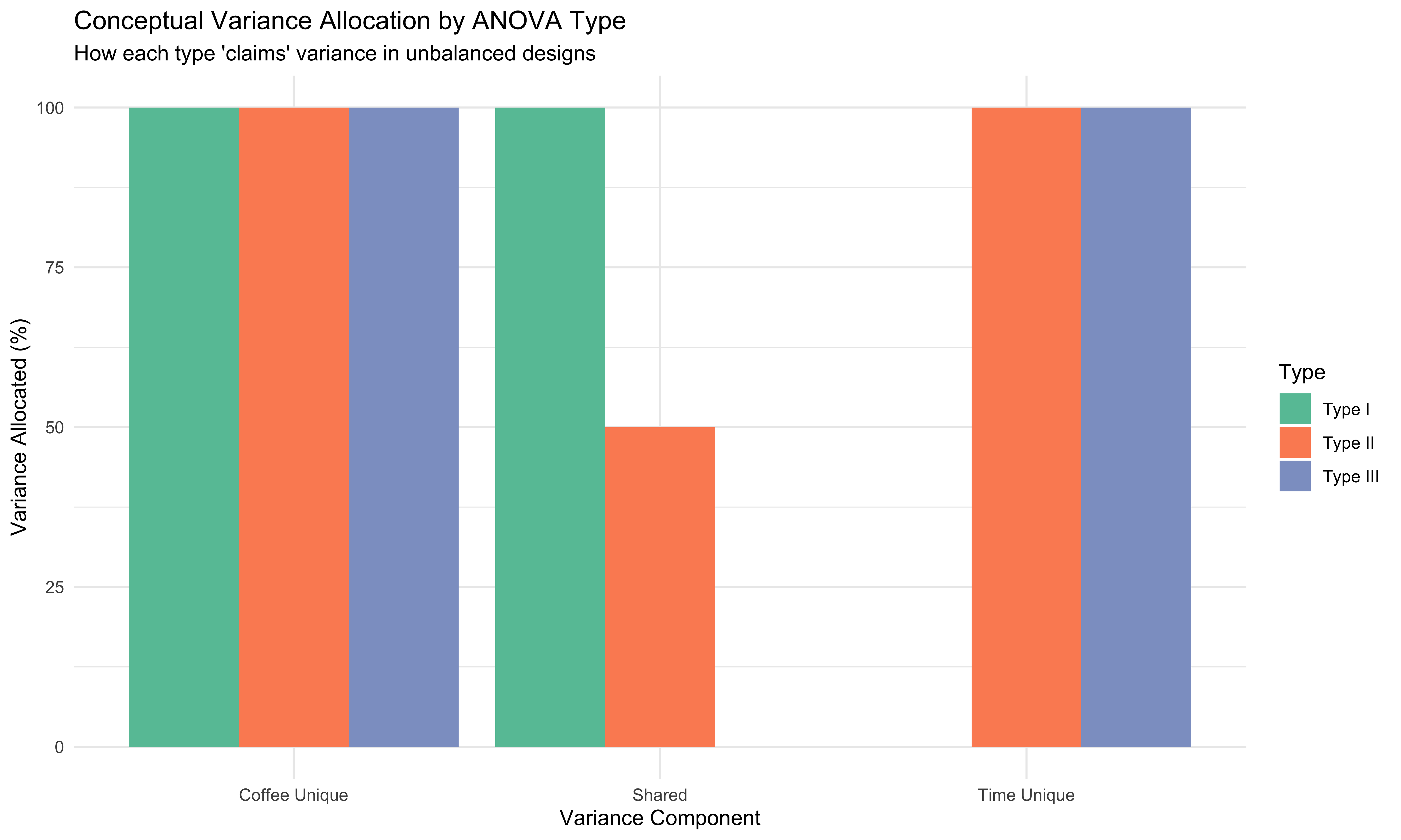

Final Recommendations Table

final_recommendations <- data.frame(
  `Research Question` = c(
    "Do factors A and B affect the outcome?",
    "What is the unique contribution of A?",
    "Does A matter after controlling for everything?",
    "Following a causal chain A→B→C",
    "Interaction is significant"
  ),
  `Best Type` = c(
    "Type II",
    "Type II",
    "Type III",
    "Type I",
    "Type III"
  ),
  `Why` = c(
    "Tests main effects properly without assuming interaction",
    "Type II isolates unique variance of each factor",
    "Type III is most conservative, controls for all",
    "Type I respects the sequential nature",
    "Type III tests main effects in presence of interaction"
  ),
  check.names = FALSE
)

kable(final_recommendations,
      caption = "Final Recommendations for ANOVA Type Selection") %>%
  kable_styling(bootstrap_options = c("striped", "hover", "condensed"))

Final Recommendations for ANOVA Type Selection

Research Question	Best Type	Why
Do factors A and B affect the outcome?	Type II	Tests main effects properly without assuming interaction
What is the unique contribution of A?	Type II	Type II isolates unique variance of each factor
Does A matter after controlling for everything?	Type III	Type III is most conservative, controls for all
Following a causal chain A→B→C	Type I	Type I respects the sequential nature
Interaction is significant	Type III	Type III tests main effects in presence of interaction

Remember this Above All

The Golden Rule of ANOVA Types

If your design is balanced, rejoice! All types give the same answer.

If your design is unbalanced:

• 1. Check if interaction is significant
• 2. If NO interaction → Use Type II
• 3. If YES interaction → Use Type III
• 4. If natural hierarchy → Consider Type I

Always report: Which type you used and why!

Appendix: R Package Requirements

# Required packages for this tutorial
required_packages <- c(
  "tidyverse",     # Data manipulation and visualization
  "car",           # For Type II and III ANOVA
  "emmeans",       # Estimated marginal means
  "knitr",         # For tables
  "kableExtra",    # Enhanced tables
  "patchwork",     # Combining plots
  "corrplot",      # Correlation plots
  "rstatix"        # Additional statistical tests
)

# Install if needed
install.packages(required_packages)

Citation

BibTeX citation:

@online{rasheduzzaman2025,
  author = {Md Rasheduzzaman},
  title = {Statistics {Basics}},
  date = {2025-09-23},
  langid = {en},
  abstract = {Statistical tests, Statistics, Statistic, CLT, etc.}
}

For attribution, please cite this work as:

Md Rasheduzzaman. 2025. “Statistics Basics.” September 23, 2025.